Confounding SHAP: Attributing Bias to Covariates

This example shows how to use the GlobalConfoundingXAI game to attribute confounding bias in a treatment effect estimate to individual covariates via Shapley values.

The Confounding XAI game defines a coalition value v(S) that measures how much confounding bias remains when a treatment effect estimator only observes feature subset S. Shapley values then decompose that bias across all features.

We use the load_curthvds_synthetic() dataset, a synthetic observational study with known ground-truth causal roles:

• Instrument: affects treatment assignment but not the outcome directly.

• Confounder: affects both treatment assignment and outcome (source of bias).

• EffectModifier: only modifies the treatment effect size.

• OutcomeOnly: affects the outcome but not treatment assignment.

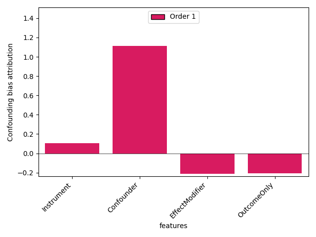
After computing Shapley values we expect the Confounder to receive the largest absolute attribution.

from __future__ import annotations

import numpy as np
from tabpfn import TabPFNRegressor

import shapiq
from shapiq_games.benchmark.causal_xai import GlobalConfoundingXAI
from shapiq_games.datasets import load_curthvds_synthetic

_TABPFN_INFERENCE_CONFIG = {"REGRESSION_Y_PREPROCESS_TRANSFORMS": (None,)}

/home/docs/checkouts/readthedocs.org/user_builds/shapiq/checkouts/latest/examples/causal/plot_confounding_xai.py:31: DeprecationWarning: This collection of games is deprecated and will be removed in a future version.
  from shapiq_games.benchmark.causal_xai import GlobalConfoundingXAI

Load Data

The Curth-VDS dataset is a synthetic observational study with four covariates. Treatment assignment is confounded by the Confounder variable.

curthvds_data = load_curthvds_synthetic(n=200, d=4, seed=42)
print(curthvds_data.head())
print(f"\nDataset shape: {curthvds_data.shape}")
print(f"Treatment rate: {curthvds_data['Treatment'].mean():.2f}")

feature_cols = [c for c in curthvds_data.columns if c not in {"Treatment", "Outcome"}]
X = curthvds_data[feature_cols].to_numpy()
A = curthvds_data["Treatment"].to_numpy()
Y = curthvds_data["Outcome"].to_numpy()

   Instrument  Confounder  EffectModifier  OutcomeOnly  Treatment   Outcome
0   -0.179611    0.304717        0.337575     0.515410          0  0.711221
1    0.196776   -1.039984        1.407482    -0.577539          1  4.162946
2    0.820528    0.750451        0.090585     1.274447          1  2.316776
3   -0.393741    0.940565        0.643939    -0.627588          1  1.823949
4    0.521167   -1.951035       -2.050172    -0.636615          1  9.238776

Dataset shape: (200, 6)
Treatment rate: 0.53

Estimate CATE with an S-Learner

We use a single TabPFN S-learner trained on the full dataset with treatment A appended as a feature. Predicting twice — once with A set to 1 and once with A set to 0 — gives the individual treatment effect estimate tau_hat. This matches the estimator used inside CurthVDS.

model = TabPFNRegressor(
    device="cpu",
    n_estimators=1,
    n_jobs=1,
    inference_config=_TABPFN_INFERENCE_CONFIG,
)
XA = np.concatenate([X, A.reshape(-1, 1)], axis=1)
model.fit(XA, Y)
XA1 = np.concatenate([X, np.ones((len(X), 1))], axis=1)
XA0 = np.concatenate([X, np.zeros((len(X), 1))], axis=1)
tau_hat = model.predict(XA1) - model.predict(XA0)

print(f"\nMean estimated CATE: {tau_hat.mean():.3f}")
print(f"Observed outcome difference: {Y[A == 1].mean() - Y[A == 0].mean():.3f}")

/home/docs/checkouts/readthedocs.org/user_builds/shapiq/checkouts/latest/examples/causal/plot_confounding_xai.py:60: DeprecationWarning: TabPFNRegressor(n_jobs=...) is deprecated and has no effect. Use `n_preprocessing_jobs` instead.
  model = TabPFNRegressor(
Warning: You are sending unauthenticated requests to the HF Hub. Please set a HF_TOKEN to enable higher rate limits and faster downloads.

Mean estimated CATE: 0.487
Observed outcome difference: 1.287

Define the Global Confounding XAI Game

The game’s value function v(S) measures the confounding bias when only the features in S are observed. For mode='signed' a positive value means the naive estimator (using only S) over-estimates the true effect.

game = GlobalConfoundingXAI(X, A, Y, tau_hat, mode="signed", device="cpu")
print(f"\nEmpty coalition value v({{}}): {game.empty_value:.4f}")
print(f"Grand coalition value v(N): {game.grand_coalition_value:.4f}")

Empty coalition value v({}): -0.8005
Grand coalition value v(N): -0.0000

Compute Exact Shapley Values

For a small game (d=4) we can enumerate all 2^4 = 16 coalitions exactly.

exact_computer = shapiq.ExactComputer(n_players=game.n_players, game=game)
sv = exact_computer(index="SV", order=1)
print(sv)

InteractionValues(
    index=SV, max_order=1, min_order=0, estimated=False, estimation_budget=None,
    n_players=4, baseline_value=-0.8005180845240998,
    Top 10 interactions:
        (1,): 1.1136284845140514
        (0,): 0.1054659264663296
        (3,): -0.20513761770556993
        (2,): -0.21343871128390857
        (): -0.8005180845240998
)

Visualize: Stacked Bar Plot

The Confounder is expected to receive the largest attribution.

sv.plot_stacked_bar(feature_names=feature_cols, ylabel="Confounding bias attribution")