Visualization Catalog

A comprehensive tour of all local and global visualization functions in shapiq: force plot, waterfall plot, network plot, SI graph plot, stacked bar plot, and global bar plot.

All examples use the same XGBoost model on the California housing dataset for consistency with the other visualization gallery scripts.

from __future__ import annotations

from sklearn.model_selection import train_test_split
from xgboost import XGBRegressor

import shapiq

Train Model and Compute Explanations

We train an XGBoost regressor and compute Shapley values (order 1) and k-SII interactions (order 2) for a single instance.

x_data, y_data = shapiq.datasets.load_california_housing(to_numpy=False)
feature_names = list(x_data.columns)
x_data, y_data = x_data.values, y_data.values
x_train, x_test, y_train, y_test = train_test_split(
    x_data,
    y_data,
    test_size=0.2,
    random_state=42,
)
model = XGBRegressor(random_state=42, max_depth=4, n_estimators=50)
model.fit(x_train, y_train)

x_explain = x_test[2]
explainer = shapiq.TabularExplainer(
    model,
    data=x_test,
    index="k-SII",
    max_order=2,
    random_state=42,
)
iv = explainer.explain(x_explain, budget=200)

sv = iv.get_n_order(1)
print(iv)

InteractionValues(
    index=k-SII, max_order=2, min_order=0, estimated=True, estimation_budget=200,
    n_players=8, baseline_value=2.058321475982666,
    Top 10 interactions:
        (): 2.058321475982666
        (7,): 1.3350600113103832
        (5,): 0.4500846779831734
        (6, 7): 0.2980846968500863
        (1, 7): 0.25150829991703183
        (2, 5): 0.20722694546625944
        (1,): 0.1832462712495247
        (3,): 0.16499400964618197
        (0,): -0.1686034639705406
        (6,): -0.4933280450422622
)

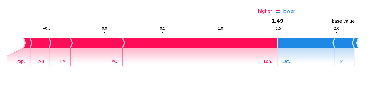
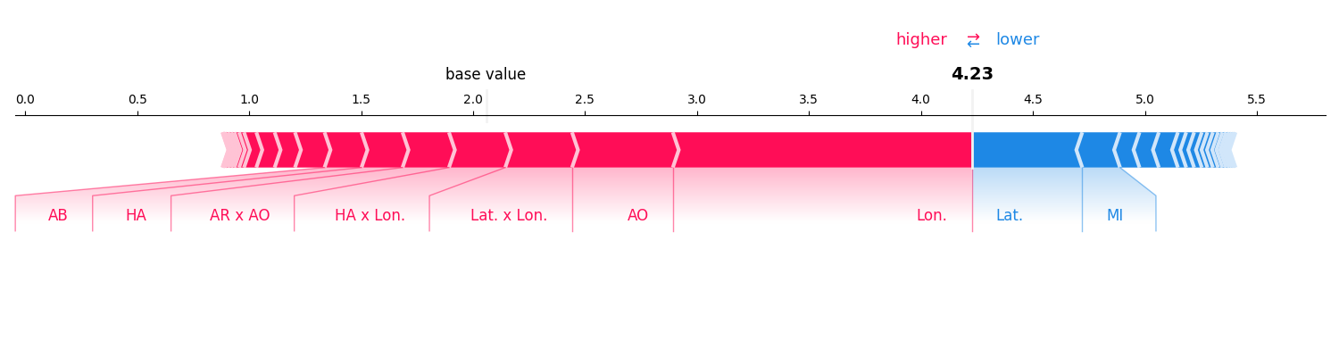
Force Plot

Shows how each interaction pushes the prediction away from the baseline. Works for any order of interactions.

sv.plot_force(feature_names=feature_names)

iv.plot_force(feature_names=feature_names)

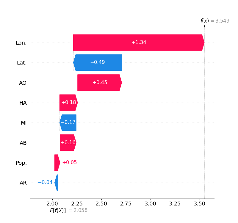
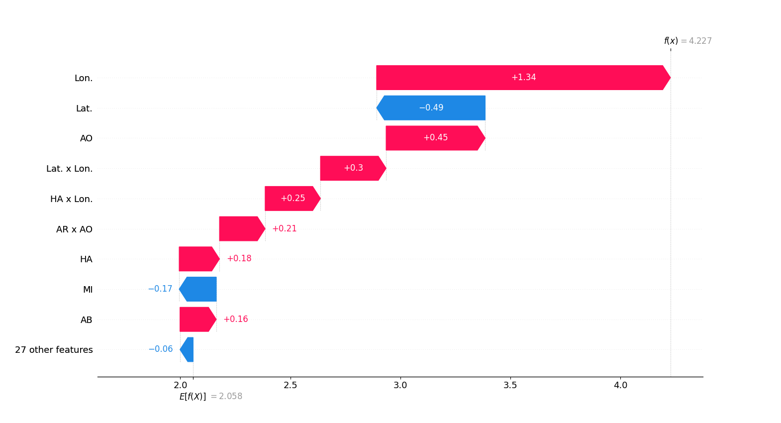
Waterfall Plot

Like the force plot but groups small interactions into an “other” bucket.

sv.plot_waterfall(feature_names=feature_names)

iv.plot_waterfall(feature_names=feature_names)

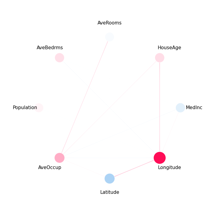
Network Plot

Visualizes first- and second-order interactions as a graph. Node size encodes first-order importance; edge width encodes pairwise interaction strength.

iv.plot_network(feature_names=feature_names)

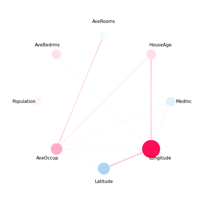
SI Graph Plot

A more general graph plot that can display higher-order interactions as hyper-edges. See the dedicated SI Graph Plot example for advanced options.

iv.plot_si_graph(feature_names=feature_names, size_factor=3.0)

Stacked Bar Plot

Shows per-feature interaction magnitude, stacked by order. Useful for comparing how much each feature contributes via main effects vs. interactions.

shapiq.stacked_bar_plot(iv.get_n_order(1), feature_names=feature_names)

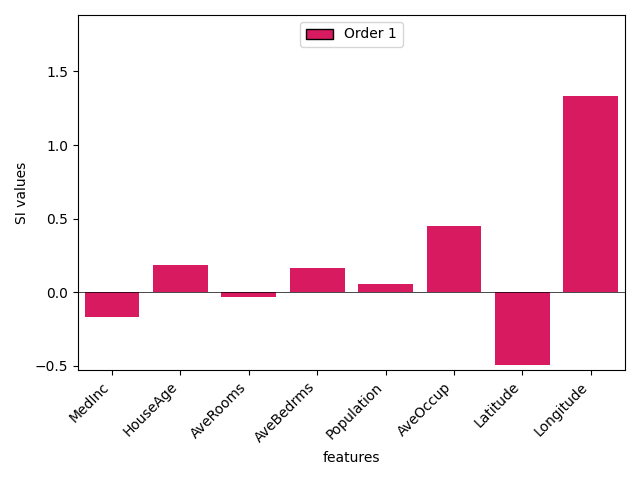
(<Figure size 640x480 with 1 Axes>, <Axes: xlabel='features', ylabel='SI values'>)

shapiq.stacked_bar_plot(iv, feature_names=feature_names)

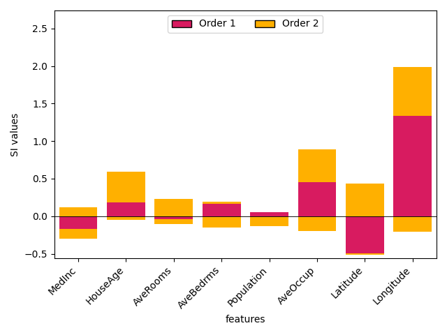
(<Figure size 640x480 with 1 Axes>, <Axes: xlabel='features', ylabel='SI values'>)

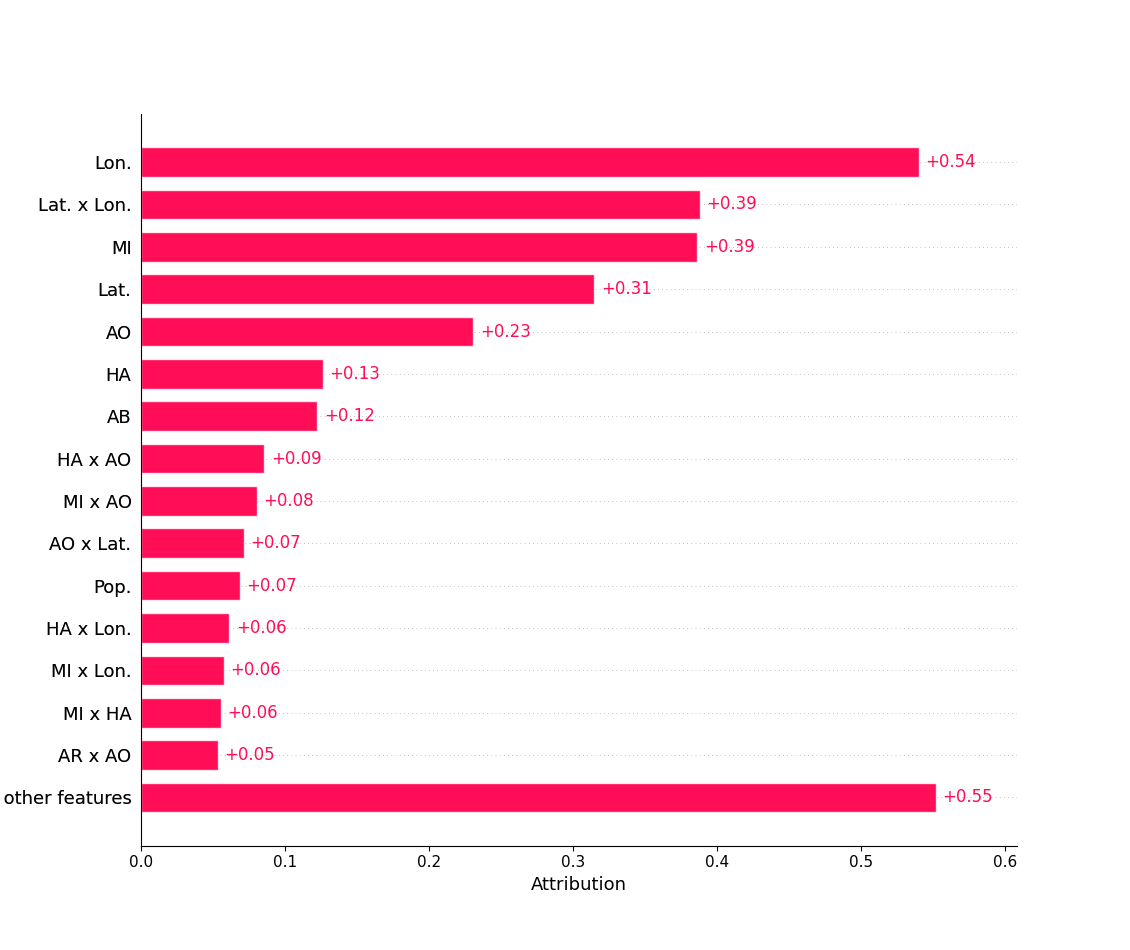
Global Bar Plot

Aggregates interaction values across multiple instances to show global feature (interaction) importance.

explanations = [explainer.explain(x_test[i], budget=200) for i in range(5)]
shapiq.plot.bar_plot(explanations, feature_names=feature_names, max_display=15)

<Axes: xlabel='Attribution'>