Explaining a Vision Transformer

This example shows how to explain an image classification by a Vision Transformer (ViT) using shapiq. The image is divided into patches and each patch becomes a player in a cooperative game. Shapley values then quantify how much each patch contributes to the predicted class.

We use the ImageClassifierLocalXAI game from the shapiq_games package, which wraps a pretrained ViT model and handles patch masking internally.

from __future__ import annotations

import os

# Prevent OpenMP/MKL thread conflicts with PyTorch backend
os.environ.setdefault("OMP_NUM_THREADS", "1")
os.environ.setdefault("MKL_NUM_THREADS", "1")

import tempfile
from pathlib import Path

import numpy as np
from PIL import Image

import shapiq
from shapiq_games.benchmark import ImageClassifierLocalXAI

Set Up the Image Game

We use a ViT model with a 3x3 grid (9 patches). Each patch is a player in the cooperative game. The game value for a coalition is the model’s predicted probability for the top class when only those patches are visible.

We create a synthetic image here for portability. In practice you would pass the path to a real photograph.

rng = np.random.default_rng(42)
image = Image.fromarray(rng.integers(0, 255, (384, 384, 3), dtype=np.uint8))
image_path = str(Path(tempfile.gettempdir()) / "shapiq_vit_example.png")
image.save(image_path)

game = ImageClassifierLocalXAI(
    model_name="vit_9_patches",
    x_explain_path=image_path,
    normalize=True,
)
print(f"Number of patches (players): {game.n_players}")
print(f"Grand coalition value: {game.grand_coalition_value:.3f}")

Loading weights:   0%|          | 0/200 [00:00<?, ?it/s]
Loading weights: 100%|██████████| 200/200 [00:00<00:00, 16312.95it/s]
Number of patches (players): 9
Grand coalition value: 0.037

Compute Shapley Values

With 9 patches we use KernelSHAP with a small budget.

approx = shapiq.KernelSHAP(n=game.n_players, random_state=42)
sv = approx.approximate(budget=50, game=game)
print(sv)

InteractionValues(
    index=SV, max_order=1, min_order=0, estimated=True, estimation_budget=50,
    n_players=9, baseline_value=0.0,
    Top 10 interactions:
        (2,): 0.011702385421281295
        (8,): 0.008703247937980616
        (6,): 0.006998279153967865
        (3,): 0.004834377573755647
        (4,): 0.004243905403750059
        (5,): 0.002051309384896535
        (0,): 0.0012419779204754528
        (1,): 0.0005732002928077967
        (): 0.0
        (7,): -0.003437167268523909
)

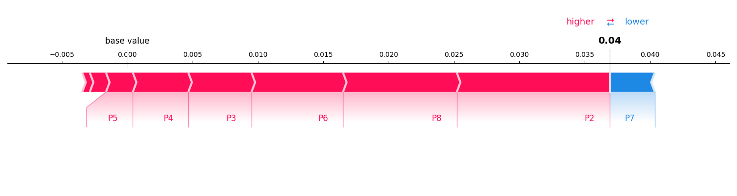
Visualize Patch Importance

A force plot shows how each patch pushes the prediction away from the baseline (all patches masked).

patch_names = [f"Patch {i}" for i in range(game.n_players)]
sv.plot_force(feature_names=patch_names)

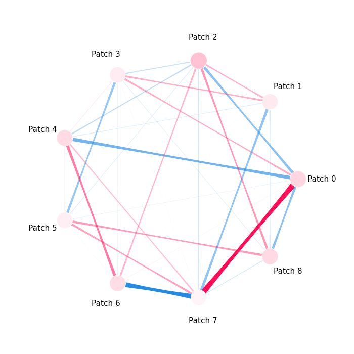
Second-Order Interactions

We can also compute pairwise interactions to see which patches interact with each other.

approx_k_sii = shapiq.KernelSHAPIQ(n=game.n_players, index="k-SII", max_order=2, random_state=42)
sii = approx_k_sii.approximate(budget=50, game=game)

sii.plot_network(feature_names=patch_names)

References