SHAP-IQ with scikit-learn

This example shows how to compute second-order Shapley Interaction Index (SII) values for a scikit-learn Random Forest on the California housing dataset.

from __future__ import annotations

from sklearn.ensemble import RandomForestRegressor
from sklearn.model_selection import train_test_split

import shapiq

Load Data and Train Model

X, y = shapiq.load_california_housing()
X_train, X_test, y_train, y_test = train_test_split(
    X.values,
    y.values,
    test_size=0.25,
    random_state=42,
)
n_features = X_train.shape[1]

model = RandomForestRegressor(
    n_estimators=100,
    max_depth=n_features,
    max_features=2 / 3,
    max_samples=2 / 3,
    random_state=42,
)
model.fit(X_train, y_train)
print(f"Train R2: {model.score(X_train, y_train):.4f}")
print(f"Test  R2: {model.score(X_test, y_test):.4f}")

Train R2: 0.7965
Test  R2: 0.7431

Compute Second-Order SII

TabularExplainer with index="SII" and max_order=2 computes pairwise Shapley interaction values.

explainer = shapiq.TabularExplainer(model=model, data=X_train, index="SII", max_order=2)
x = X_test[24]
iv = explainer.explain(x, budget=2**n_features, random_state=0)
print(iv)

InteractionValues(
    index=SII, max_order=2, min_order=0, estimated=False, estimation_budget=256,
    n_players=8, baseline_value=2.0701874006108745,
    Top 10 interactions:
        (6,): 0.1478250584673519
        (1, 5): 0.10379041749007883
        (5, 6): -0.03359635591281193
        (6, 7): -0.0442855087946712
        (0, 1): -0.04664913270961242
        (0, 6): -0.052169397474938504
        (1,): -0.080623853044805
        (0, 5): -0.08271510620749073
        (5,): -0.14868378081300276
        (7,): -0.25600704535637764
)

Second-Order Interaction Matrix

print(iv.get_n_order(2).dict_values)

{(0, 1): -0.04664913270961242, (0, 2): 0.014949695697994765, (0, 3): -0.0257174179766264, (0, 4): -0.021236779745596106, (0, 5): -0.08271510620749073, (0, 6): -0.052169397474938504, (0, 7): 0.006477294716412733, (1, 2): -0.01360457048275386, (1, 3): -0.019193609392757372, (1, 4): -0.018151921305244546, (1, 5): 0.10379041749007883, (1, 6): -0.02162920040812735, (1, 7): -0.025722171014265955, (2, 3): -0.02003480515133269, (2, 4): -0.020121478625975835, (2, 5): -0.020934613059505128, (2, 6): -0.01757370947785476, (2, 7): -0.025719160762024858, (3, 4): -0.020781921700697314, (3, 5): -0.01570798766795791, (3, 6): -0.024584796522633824, (3, 7): -0.022438636770326228, (4, 5): -0.02418830404440444, (4, 6): -0.021910782841727837, (4, 7): -0.01970633212232046, (5, 6): -0.03359635591281193, (5, 7): -0.006788344815203122, (6, 7): -0.0442855087946712}

Visualization: Network Plot

shapiq.network_plot(interaction_values=iv, feature_names=list(X.columns))

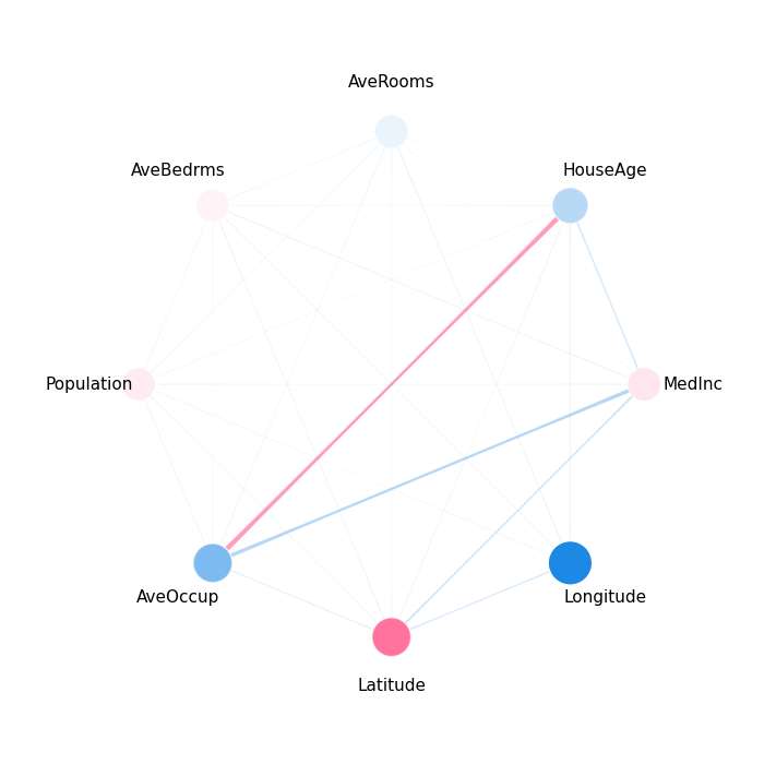
(<Figure size 700x700 with 1 Axes>, <Axes: >)

Stacked Bar Plot (First Order)

shapiq.stacked_bar_plot(iv.get_n_order(1), feature_names=list(X.columns))

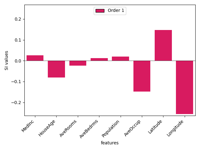
(<Figure size 640x480 with 1 Axes>, <Axes: xlabel='features', ylabel='SI values'>)

Stacked Bar Plot (All Orders)

shapiq.stacked_bar_plot(interaction_values=iv, feature_names=list(X.columns))

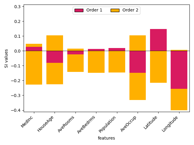
(<Figure size 640x480 with 1 Axes>, <Axes: xlabel='features', ylabel='SI values'>)

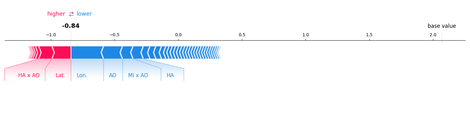
Force Plot

iv.plot_force(feature_names=list(X.columns))