Conditional Data Imputation

This example shows how to use ConditionalImputer for conditional (observational) imputation when computing Shapley interactions. Conditional imputation respects feature dependencies, unlike marginal (interventional) imputation.

from __future__ import annotations

from sklearn.ensemble import RandomForestRegressor
from sklearn.model_selection import train_test_split

import shapiq

Load Data and Train Model

X, y = shapiq.load_california_housing()
X_train, X_test, y_train, y_test = train_test_split(
    X.values,
    y.values,
    test_size=0.25,
    random_state=42,
)
n_features = X_train.shape[1]

model = RandomForestRegressor(
    n_estimators=100,
    max_depth=n_features,
    max_features=2 / 3,
    max_samples=2 / 3,
    random_state=42,
)
model.fit(X_train, y_train)
print(f"Train R2: {model.score(X_train, y_train):.4f}")
print(f"Test  R2: {model.score(X_test, y_test):.4f}")

Train R2: 0.7965
Test  R2: 0.7431

Conditional Imputer

Set imputer="conditional" in TabularExplainer. The imputer trains a gradient boosting model per feature to learn the conditional distribution. Key parameters:

• sample_size: samples drawn from conditional background

• conditional_budget: coalitions per data point for training

• conditional_threshold: quantile threshold for neighbourhood

explainer = shapiq.TabularExplainer(
    model=model,
    data=X_train,
    index="SII",
    max_order=2,
    imputer="conditional",
    sample_size=100,
    conditional_budget=32,
    conditional_threshold=0.04,
)

Explain a Single Instance

x_explain = X_test[100]
iv = explainer.explain(x_explain, budget=2**n_features, random_state=0)
print(iv)

InteractionValues(
    index=SII, max_order=2, min_order=0, estimated=False, estimation_budget=256,
    n_players=8, baseline_value=2.0701874006108745,
    Top 10 interactions:
        (0, 1): 0.07235594319404895
        (5,): 0.06398005281148228
        (2,): 0.037374147027905556
        (5, 7): 0.037311123046789234
        (1, 7): -0.029679463654197765
        (1, 5): -0.0336762113531598
        (0, 7): -0.06493048753501021
        (1,): -0.1331566617040377
        (7,): -0.17584970197462807
        (0,): -0.19972672348833737
)

Network Plot

shapiq.network_plot(interaction_values=iv, feature_names=list(X.columns))

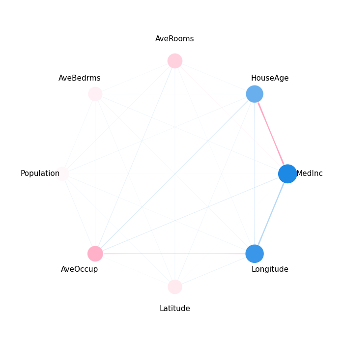
(<Figure size 700x700 with 1 Axes>, <Axes: >)