Data Valuation with Nearest Neighbor Explainers

This notebook shows how explainers of nearest-neighbor (NN) models can be used for Data Valuation, the task of evaluating the usefulness of individual training data points in classification problems. When explaining NN models, a game is defined by first choosing an explanation point \(x_\text{explain}\) and class \(y_\text{explain}\); the training data points \(\mathcal{D} := \mathcal{X} \times \mathcal{Y}\) are the game’s players, and the definition of the utility \(\nu(S)\) of a coalition \(S \subseteq \mathcal{D}\) is based on the probability of the model predicting class \(y_\text{explain}\) on \(x_\text{explain}\) if it’s training data were limited to \(S\).

There is support for explaining the the KNeighborsClassifier model (with 'uniform' or 'distance' weights) and RadiusNeighborsClassifier model from the scikit-learn library. The algorithms are based on the publications from Jia et al. (2019), Wang et al. (2024) and Wang et al. (2023), respectively.

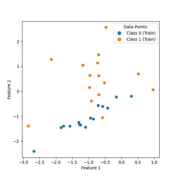
Let’s start by generating a synthetic classification datset and fitting a simple KNeighborsClassifier to it.

import matplotlib.pyplot as plt
import numpy as np
from sklearn.datasets import make_classification
from sklearn.neighbors import KNeighborsClassifier, RadiusNeighborsClassifier
from util_plot import plot_datasets

X_train, y_train = make_classification(
    n_samples=30,
    n_features=2,
    n_redundant=0,
    n_clusters_per_class=1,
    n_informative=2,
    n_classes=2,
    random_state=45,
)

fig, ax = plt.subplots(figsize=(6, 6))
plot_datasets(ax, X_train, y_train)

model = KNeighborsClassifier(n_neighbors=3)
model.fit(X_train, y_train)

x_explain = np.array([[-0.75, -0.4]])
y_explain_pred = model.predict(x_explain)[0]
print(f"Prediction: class {y_explain_pred}")

y_explain_proba = model.predict_proba(x_explain)[0]
print(f"Prediction probabilities: {y_explain_proba}")

Prediction: class 0
Prediction probabilities: [0.66666667 0.33333333]

Using the KNNExplainer for Unweighted \(k\)-Nearest Neighbor Models

To explain the prediction, we create an explainer for the model by passing it to the constructor of Explainer, which will automatically dispatch to the adequate subclass KNNExplainer.

from shapiq import Explainer

explainer = Explainer(model, class_index=y_explain_pred, index="SV", max_order=1)
print(type(explainer))

<class 'shapiq.explainer.nn.knn.KNNExplainer'>

Note that we set class_index=y_explain_pred, since for now, we want to quantify the contribution of the training data to the class that was actually predicted. (We could also set a different class index if we wished to see how much the data points contribute to shifting the prediction towards another class.)

Now we can get an explanation for the prediction we saw above:

iv = explainer.explain(x_explain)
print(iv)

InteractionValues(
    index=SV, max_order=1, min_order=0, estimated=True, estimation_budget=None,
    n_players=30, baseline_value=0,
    Top 10 interactions:
        (9,): 0.20212345126138226
        (23,): 0.20212345126138226
        (2,): 0.11879011792804894
        (14,): 0.08545678459471562
        (15,): 0.06759964173757277
        (28,): 0.06759964173757277
        (16,): 0.058508732646663675
        (19,): -0.08120988207195104
        (1,): -0.13120988207195106
        (4,): -0.13120988207195106
)

Explaining Weighted \(k\)-Nearest Neighbor and Threshold Nearest Neighbor Models

There are separate explainers for weighted \(k\)-NN and threshold NN models, which are selected automatically when an Explainer is instantiated with a corresponding model:

wknn_model = KNeighborsClassifier(n_neighbors=3, weights="distance")
wknn_model.fit(X_train, y_train)
wknn_explainer = Explainer(wknn_model, class_index=0, index="SV", max_order=1)
print(type(wknn_explainer))

tnn_model = RadiusNeighborsClassifier()
tnn_model.fit(X_train, y_train)
tnn_explainer = Explainer(tnn_model, class_index=0, index="SV", max_order=1)
print(type(tnn_explainer))

<class 'shapiq.explainer.nn.weighted_knn.WeightedKNNExplainer'>
<class 'shapiq.explainer.nn.threshold_nn.ThresholdNNExplainer'>

They can be used just the same way:

print(wknn_explainer.explain(x_explain))
print(tnn_explainer.explain(x_explain))

InteractionValues(
    index=SV, max_order=1, min_order=0, estimated=True, estimation_budget=None,
    n_players=30, baseline_value=0,
    Top 10 interactions:
        (23,): 0.5414010940326729
        (9,): 0.4580677606993394
        (2,): 0.1858067858067858
        (14,): 0.09743098032571718
        (15,): 0.08314526604000289
        (28,): 0.08314526604000289
        (21,): -0.06915214415214416
        (19,): -0.09058071558071559
        (1,): -0.2653449377133588
        (4,): -0.3752655726339937
)
InteractionValues(
    index=SV, max_order=1, min_order=0, estimated=True, estimation_budget=None,
    n_players=30, baseline_value=0,
    Top 10 interactions:
        (): 0.5
        (2,): 0.13726715203987933
        (14,): 0.13726715203987933
        (15,): 0.13726715203987933
        (23,): 0.13726715203987933
        (1,): -0.1556296733569461
        (4,): -0.1556296733569461
        (17,): -0.1556296733569461
        (19,): -0.1556296733569461
        (21,): -0.1556296733569461
)

Large numbers of training samples

Since the algorithms are pretty efficient, we can run them on large sets of training data.

from time import time


def print_explain_times(model, n, n_test) -> None:
    X_train, y_train = make_classification(
        n_samples=n,
        n_features=5,
        n_redundant=0,
        n_clusters_per_class=1,
        n_informative=3,
        n_classes=2,
        random_state=45,
    )
    X_test = X_train[:n_test]
    X_train = X_train[n_test:]
    y_train = y_train[n_test:]
    model.fit(X_train, y_train)
    explainer = Explainer(model, class_index=0, index="SV", max_order=1)

    times = np.zeros((n_test,))
    for i, x_test in enumerate(X_test):
        t_start = time()
        explainer.explain(x_test)
        t_end = time()
        times[i] = t_end - t_start
    mean = np.mean(times) * 1000
    std = np.std(times) * 1000
    print(f"{explainer.__class__.__name__} on {n} samples: average {mean:.1f}±{std:.1f}ms")

The cell below which uses the KNN explainer takes roughly 0.15 s to explain a single data point on a consumer-grade laptop with a 12th Gen Intel i5 processor.

print_explain_times(KNeighborsClassifier(n_neighbors=5, weights="uniform"), n=100_000, n_test=50)

KNNExplainer on 100000 samples: average 151.3±1.2ms

Since the algorithm of the WKNN explainer is less efficient, featuring a quadratic runtime complexity, the number of data points needs to be limited.

print_explain_times(KNeighborsClassifier(n_neighbors=5, weights="distance"), n=200, n_test=10)

WeightedKNNExplainer on 200 samples: average 1843.1±6.2ms

The TNN algorithm, on the other hand, is faster:

print_explain_times(RadiusNeighborsClassifier(radius=5), n=100_000, n_test=50)

ThresholdNNExplainer on 100000 samples: average 66.8±1.0ms

## Identifying corrupted training samples

We can estimate the usefulness of each point of a training datset by calculating Shapley values for a set of test data points and averaging the results. This will allow us to identify potentially mislabeled data points.

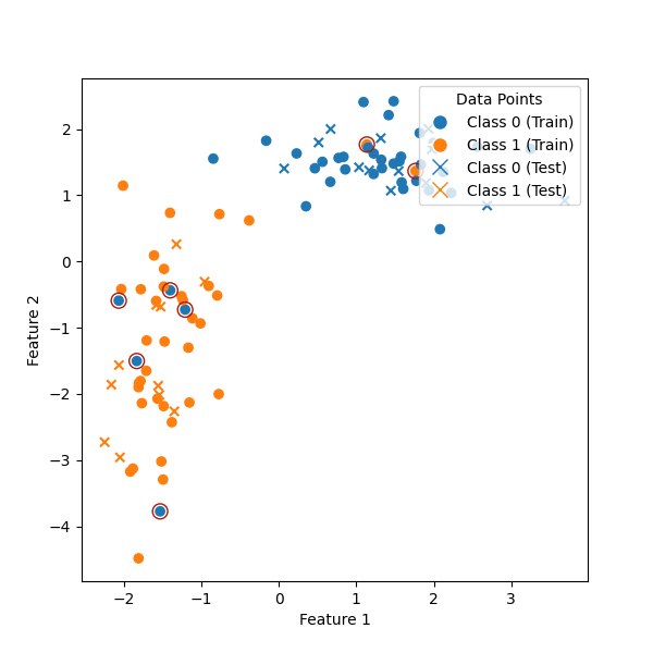
First, let’s create a classification datset and split it into train and test sets. We will corrupt the training data by changing the class of a few randomly selected data points.

from sklearn.model_selection import train_test_split

X, y = make_classification(
    n_samples=100,
    n_features=2,
    n_redundant=0,
    n_clusters_per_class=1,
    n_informative=2,
    n_classes=2,
    flip_y=0,
    random_state=49,
    class_sep=1.5,
)

X_train, X_test, y_train, y_test = train_test_split(X, y, test_size=0.25, random_state=42)

y_train_corrupted = y_train.copy()
n_corrupt = 7
rng = np.random.default_rng(seed=43)
corrupted = rng.choice(np.arange(X_train.shape[0]), size=n_corrupt, replace=False)
# Since our only class indices are 0 and 1, this is a quick way to flip the class
y_train_corrupted[corrupted] = 1 - y_train[corrupted]

fig, ax = plt.subplots(figsize=(6, 6))
plot_datasets(ax, X_train, y_train_corrupted, X_test, y_test)
# Mark corrupted datapoints
ax.scatter(
    X_train[corrupted, 0],
    X_train[corrupted, 1],
    marker="o",
    edgecolors="#b1170c",
    facecolors="none",
    s=100,
)

<matplotlib.collections.PathCollection object at 0x731d41855f40>

Now, we can use the KNNExplainer to compute the training points’ Shapley values based on the entire test dataset by averaging the Shapley values computed using each test point.

# Train the model with the corrupted training data
model = KNeighborsClassifier(n_neighbors=5)
model.fit(X_train, y_train_corrupted)

sv_test = np.zeros(X_train.shape[0], dtype=np.float64)

for x_test_current, y_test_current in zip(X_test, y_test, strict=True):
    explainer = Explainer(model, class_index=y_test_current, index="SV", max_order=1)
    iv = explainer.explain(x_test_current)
    sv_test += iv.to_first_order_array()

sv_test /= X_test.shape[0]

We can reasonably assume that the corrupted training data points will on average make the model’s prediction worse, resulting in negative Shapley values. So let’s filter out just those indices where the Shapley value is below zero and compare with our original array of corrupted indices:

print(f"Corrupted: {np.sort(corrupted)}")  # Sort for easier comparison
print(f"Negative Shapley values: {np.where(sv_test < 0)[0]}")

Corrupted: [ 1  3 20 28 34 42 45]
Negative Shapley values: [ 1  3 28 34 42 45]

We have identified the set corrupted samples almost exactly.