TreeSHAP-IQ for LightGBM

This example demonstrates TreeExplainer on a LightGBM model trained on the bike-sharing dataset. The explainer computes exact any-order Shapley interaction values for tree ensembles, as introduced by TreeSHAP-IQ, via the numerically exact Quadrature-TreeSHAP algorithm.

from __future__ import annotations

import lightgbm
from sklearn.model_selection import train_test_split

import shapiq

Load Data and Train Model

X, y = shapiq.load_bike_sharing()
X_train, X_test, y_train, y_test = train_test_split(
    X.values,
    y.values,
    test_size=0.25,
    random_state=42,
)
n_features = X_train.shape[1]

model = lightgbm.LGBMRegressor(
    n_estimators=100,
    max_depth=n_features,
    random_state=42,
    verbose=-1,
)
model.fit(X_train, y_train)
print(f"Train R2: {model.score(X_train, y_train):.4f}")
print(f"Test  R2: {model.score(X_test, y_test):.4f}")

/home/docs/checkouts/readthedocs.org/user_builds/shapiq/checkouts/latest/.venv/lib/python3.12/site-packages/sklearn/utils/validation.py:2691: UserWarning: X does not have valid feature names, but LGBMRegressor was fitted with feature names
  warnings.warn(
Train R2: 0.9599
/home/docs/checkouts/readthedocs.org/user_builds/shapiq/checkouts/latest/.venv/lib/python3.12/site-packages/sklearn/utils/validation.py:2691: UserWarning: X does not have valid feature names, but LGBMRegressor was fitted with feature names
  warnings.warn(
Test  R2: 0.9478

Compute Shapley Interactions

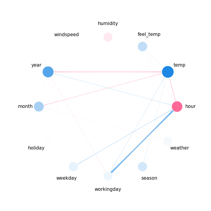
We compute k-SII scores up to order 3 for a single instance.

explainer = shapiq.TreeExplainer(model=model, index="k-SII", min_order=1, max_order=3)
x = X_test[1234]
interaction_values = explainer.explain(x)
print(interaction_values)

InteractionValues(
    index=k-SII, max_order=3, min_order=1, estimated=False, estimation_budget=None,
    n_players=12, baseline_value=190.379622526228,
    Top 10 interactions:
        (0,): 35.08515951088176
        (1, 5): 14.984490827501004
        (0, 1): 14.033445365073877
        (1, 6): 11.12425158098959
        (0, 8): -13.612044956259075
        (2,): -15.387584854862812
        (6,): -21.973797366562593
        (0, 9): -32.87403657756311
        (5,): -42.99160922657119
        (1,): -56.727108435423574
)

First-order Values (Shapley Values)

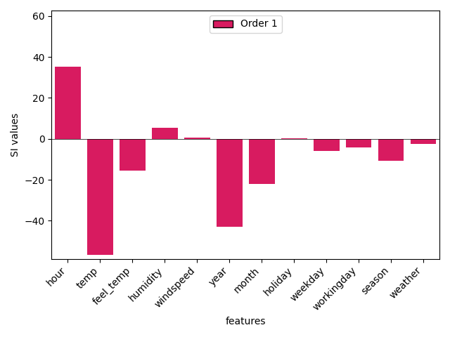
print(interaction_values.get_n_order(1).dict_values)

{(0,): 35.08515951088176, (1,): -56.727108435423574, (2,): -15.387584854862812, (3,): 5.371857243915975, (4,): 0.5157679457473102, (5,): -42.99160922657119, (6,): -21.973797366562593, (7,): 0.254449398029316, (8,): -5.9346373912897095, (9,): -4.207060851031896, (10,): -10.861061944301241, (11,): -2.4720892663115492}

Visualization: Network Plot

shapiq.network_plot(interaction_values=interaction_values, feature_names=list(X.columns))

(<Figure size 700x700 with 1 Axes>, <Axes: >)

Stacked Bar Plot (First Order)

shapiq.stacked_bar_plot(
    interaction_values=interaction_values.get_n_order(1),
    feature_names=list(X.columns),
)

(<Figure size 640x480 with 1 Axes>, <Axes: xlabel='features', ylabel='SI values'>)

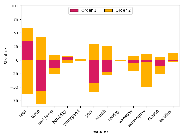
Stacked Bar Plot (First + Second Order)

shapiq.stacked_bar_plot(
    interaction_values=interaction_values.get_n_order(2, min_order=1),
    feature_names=list(X.columns),
)

(<Figure size 640x480 with 1 Axes>, <Axes: xlabel='features', ylabel='SI values'>)

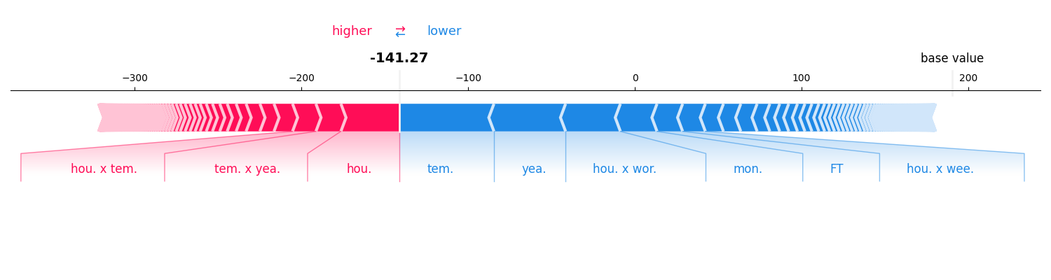
Force Plot

interaction_values.plot_force(feature_names=list(X.columns), contribution_threshold=0.03)

Global Feature Importance

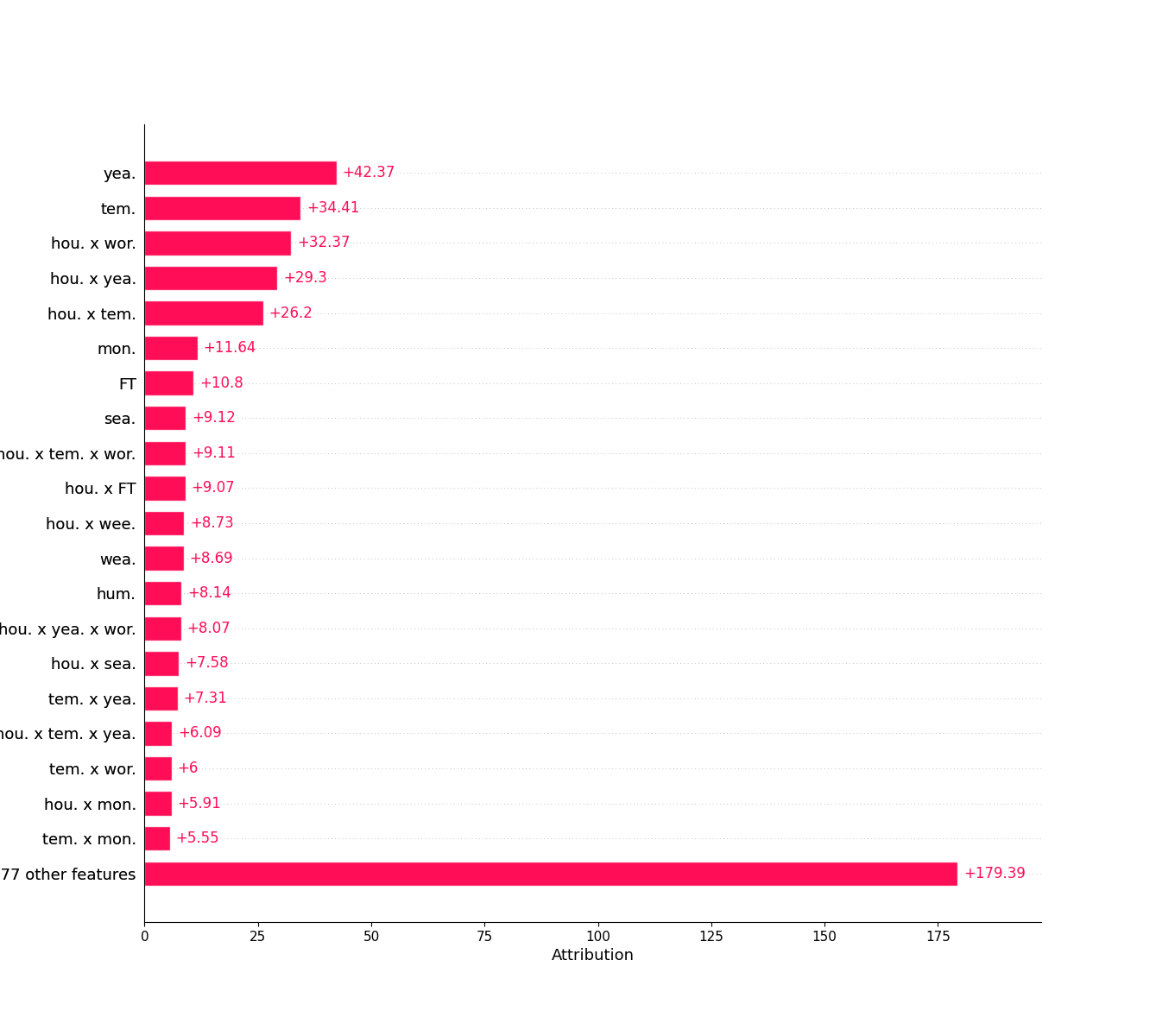
Compute interaction values for 50 test instances and show global bar plot.

list_of_ivs = explainer.explain_X(X_test[:50])
shapiq.plot.bar_plot(list_of_ivs, feature_names=list(X.columns), max_display=20)

<Axes: xlabel='Attribution'>