Explaining TabPFN¶

TabPFN is a foundation model for tabular data that uses in-context learning – fitting is just storing the training data, and inference contextualises new inputs against that context.

shapiq provides a dedicated TabPFNExplainer that exploits this property with a remove-and-recontextualize strategy: instead of imputing missing features, it simply drops feature columns from the training and test data and re-fits the model. This is both faithful to the model and inexpensive, because TabPFN’s “retraining” is just an in-context forward pass.

from __future__ import annotations

import os

# Prevent OpenMP/MKL thread conflicts with TabPFN's PyTorch backend
os.environ.setdefault("OMP_NUM_THREADS", "1")
os.environ.setdefault("MKL_NUM_THREADS", "1")

import numpy as np
from sklearn.model_selection import train_test_split

import shapiq

Prepare a Small Dataset¶

We use the California housing dataset with a tiny split so that TabPFN runs quickly on CPU.

x_data, y_data = shapiq.datasets.load_california_housing()
feature_names = list(x_data.columns)

x_train, x_test, y_train, y_test = train_test_split(
    x_data.values,
    y_data.values,
    train_size=30,
    test_size=50,
    random_state=42,
)
print(f"Train: {x_train.shape}, Test: {x_test.shape}")

Train: (30, 8), Test: (50, 8)

Fit TabPFN¶

We use TabPFNRegressor with n_estimators=1 and fit_mode="low_memory" to minimise runtime. Fitting is instant – TabPFN just stores the training context.

import tabpfn

model = tabpfn.TabPFNRegressor(
    model_path="tabpfn-v2-regressor.ckpt",
    n_estimators=1,
    fit_mode="low_memory",
)
model.fit(x_train, y_train)

avg_pred = float(np.mean(model.predict(x_test)))
print(f"Average prediction: {avg_pred:.3f}")

Average prediction: 2.086

Auto-Detection of TabPFNExplainer¶

When you pass a TabPFN model to Explainer, shapiq automatically selects TabPFNExplainer and sets up a TabPFNImputer under the hood. No special configuration is needed – just pass the model, training data, and training labels.

x_explain = x_test[0]
pred = model.predict(x_explain.reshape(1, -1))[0]
print(f"Prediction for instance: {pred:.3f}, Average: {avg_pred:.3f}")

explainer = shapiq.Explainer(
    model=model,
    data=x_train,
    labels=y_train,
    index="SV",
    max_order=1,
    empty_prediction=avg_pred,
)
print(f"Auto-selected explainer: {type(explainer).__name__}")

Prediction for instance: 0.859, Average: 2.086
Auto-selected explainer: TabPFNExplainer

How Remove-and-Recontextualize Works¶

Traditional model-agnostic explanation imputes absent features with background samples (marginal or conditional imputation). This can create out-of-distribution inputs that mislead the model.

The TabPFNImputer takes a different approach:

For each coalition \(S \subseteq \{1, \dots, d\}\) of features:
Remove the columns not in \(S\) from both training and test data.
Re-fit the TabPFN model on the reduced training data (instant, since it is just an in-context forward pass).
Predict on the reduced test point.

This faithfully reflects what the model “knows” when only features in \(S\) are available, without any distributional assumptions.

Compute Shapley Values¶

sv = explainer.explain(x_explain, budget=50)
print(sv)

sv.plot_force(feature_names=feature_names)

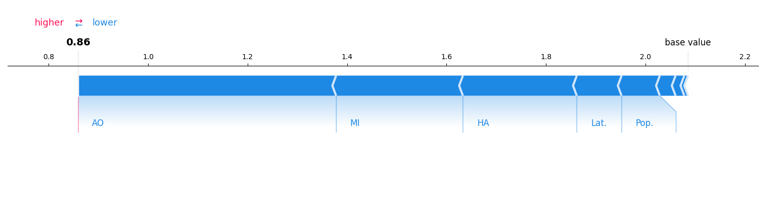
InteractionValues(
    index=SV, max_order=1, min_order=0, estimated=True, estimation_budget=50,
    n_players=8, baseline_value=2.0855908393859863,
    Top 10 interactions:
        (): 2.0855908393859863
        (2,): -0.0074234513730656645
        (7,): -0.017530992918561524
        (3,): -0.031643556722903324
        (4,): -0.07693003662491281
        (6,): -0.0900684762483492
        (1,): -0.22901624103480134
        (0,): -0.2550066261889832
        (5,): -0.5189941431956514
)

Second-Order Interactions (FSII)¶

We can also compute Faithful Shapley Interaction Index values to see which pairs of features interact.

explainer_fsii = shapiq.Explainer(
    model=model,
    data=x_train,
    labels=y_train,
    index="FSII",
    max_order=2,
    empty_prediction=avg_pred,
)
fsii = explainer_fsii.explain(x_explain, budget=50)
print(fsii)

fsii.plot_force(feature_names=feature_names)

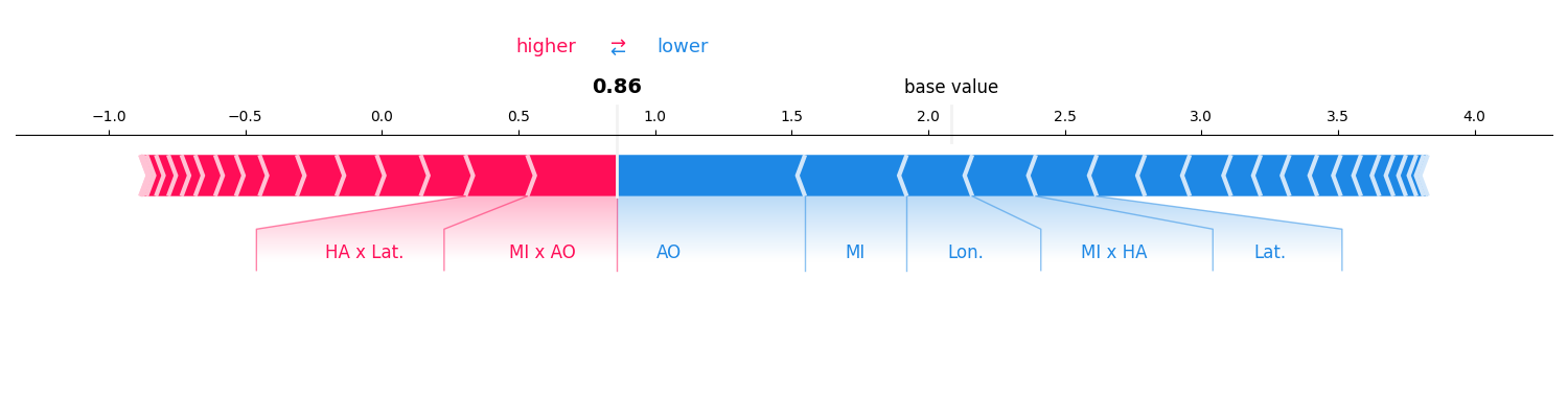
InteractionValues(
    index=FSII, max_order=2, min_order=0, estimated=True, estimation_budget=50,
    n_players=8, baseline_value=2.0855908393859863,
    Top 10 interactions:
        (): 2.0855908393859863
        (0, 5): 0.3265402343124412
        (1, 6): 0.22656658090307272
        (1, 2): -0.16400393967669868
        (0, 7): -0.17672435717262952
        (6,): -0.22271323208873753
        (0, 1): -0.2328441622485711
        (7,): -0.23996245630938012
        (0,): -0.3723259258469466
        (5,): -0.6902544586112724
)

References¶

This example uses TabPFN Hollmann et al.[1] with the remove-and-recontextualize strategy from Rundel et al.[2].

Total running time of the script: (0 minutes 17.660 seconds)