SHAP-IQ with scikit-learn

This example shows how to compute second-order Shapley Interaction Index (SII) values for a scikit-learn Random Forest on the California housing dataset.

from __future__ import annotations

from sklearn.ensemble import RandomForestRegressor
from sklearn.model_selection import train_test_split

import shapiq
from shapiq_benchmark.datasets import load_dataset

Load Data and Train Model

dataset = load_dataset("california_housing")
X, y, feature_names = dataset.x, dataset.y, list(dataset.feature_names)
X_train, X_test, y_train, y_test = train_test_split(
    X,
    y,
    test_size=0.25,
    random_state=42,
)
n_features = X_train.shape[1]

model = RandomForestRegressor(
    n_estimators=100,
    max_depth=n_features,
    max_features=2 / 3,
    max_samples=2 / 3,
    random_state=42,
)
model.fit(X_train, y_train)
print(f"Train R2: {model.score(X_train, y_train):.4f}")
print(f"Test  R2: {model.score(X_test, y_test):.4f}")

Train R2: 0.7965
Test  R2: 0.7431

Compute Second-Order SII

TabularExplainer with index="SII" and max_order=2 computes pairwise Shapley interaction values.

explainer = shapiq.TabularExplainer(
    model=model,
    data=X_train,
    sample_size=100,  # background rows the imputer averages over
    index="SII",
    max_order=2,
)
x = X_test[24]
iv = explainer.explain(x, budget=2**n_features, random_state=0)
print(iv)

InteractionValues(
    index=SII, max_order=2, min_order=0, estimated=False, estimation_budget=256,
    n_players=8, baseline_value=2.2146737291409497,
    Top 10 interactions:
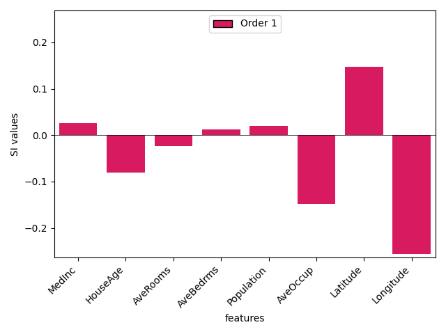
        (6,): 0.12945735684093643
        (1, 5): 0.12444616705489164
        (0, 2): 0.03560273606013122
        (0, 7): 0.02763617963550383
        (0, 6): -0.03189954070033155
        (2,): -0.041509648875587786
        (0, 5): -0.06227076139254181
        (1,): -0.09871909893850353
        (5,): -0.1671691235185329
        (7,): -0.27341469470309987
)

Second-Order Interaction Matrix

print(iv.get_n_order(2).dict_values)

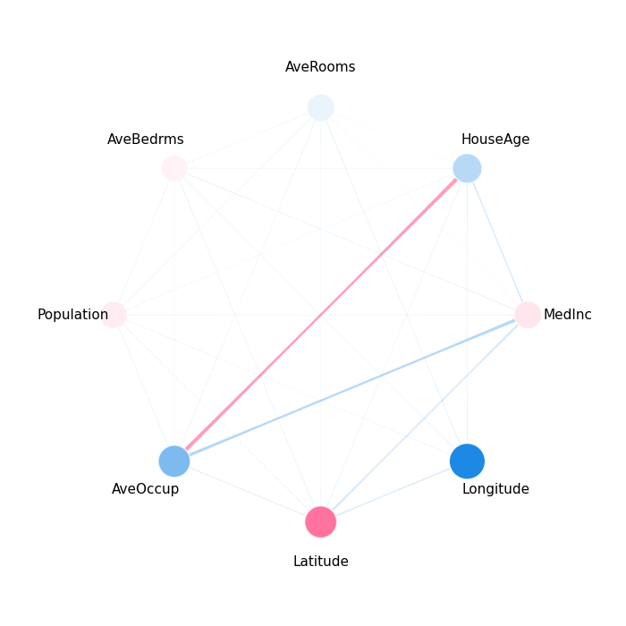
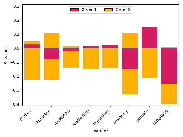
{(0, 1): -0.02595098532598578, (0, 2): 0.03560273606013122, (0, 3): -0.005097518197695498, (0, 4): -0.0005946296091558432, (0, 5): -0.06227076139254181, (0, 6): -0.03189954070033155, (0, 7): 0.02763617963550383, (1, 2): 0.007052346564437826, (1, 3): 0.0014485437763212422, (1, 4): 0.002490233023178037, (1, 5): 0.12444616705489164, (1, 6): -0.0011201369861549015, (1, 7): -0.004999256757306132, (2, 3): 0.0006073483675540445, (2, 4): 0.000520672243824666, (2, 5): -0.000358483485554412, (2, 6): 0.0030171767625164015, (2, 7): -0.004926313427043049, (3, 4): -0.00013976255873152536, (3, 5): 0.004911912493708124, (3, 6): -0.003942633094649492, (3, 7): -0.0017853540206791455, (4, 5): -0.003546146829372825, (4, 6): -0.0012686181158660986, (4, 7): 0.0009358189083710673, (5, 6): -0.01156387973309765, (5, 7): 0.012735985119914384, (6, 7): -0.02490230795260718}

Visualization: Network Plot

shapiq.network_plot(interaction_values=iv, feature_names=feature_names)

(<Figure size 700x700 with 1 Axes>, <Axes: >)

Stacked Bar Plot (First Order)

shapiq.stacked_bar_plot(iv.get_n_order(1), feature_names=feature_names)

(<Figure size 640x480 with 1 Axes>, <Axes: xlabel='features', ylabel='SI values'>)

Stacked Bar Plot (All Orders)

shapiq.stacked_bar_plot(interaction_values=iv, feature_names=feature_names)

(<Figure size 640x480 with 1 Axes>, <Axes: xlabel='features', ylabel='SI values'>)

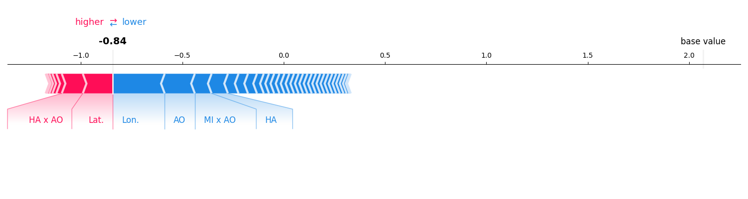
Force Plot

iv.plot_force(feature_names=feature_names)