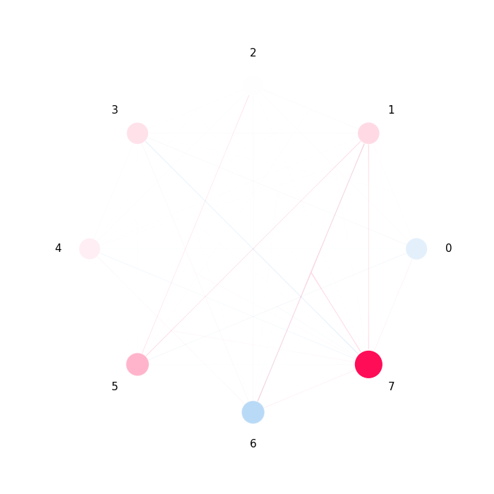
SI Graph Plot

This example demonstrates the SI graph plot, which visualizes Shapley interactions as a network. Players are nodes; interactions are edges whose color, thickness, and opacity encode strength and direction.

from __future__ import annotations

from sklearn.model_selection import train_test_split
from xgboost import XGBRegressor

import shapiq

Train a Model

We use an XGBoost regressor on the California housing dataset.

x_data, y_data = shapiq.datasets.load_california_housing(to_numpy=False)
feature_names = list(x_data.columns)
x_data, y_data = x_data.values, y_data.values
x_train, x_test, y_train, y_test = train_test_split(
    x_data,
    y_data,
    test_size=0.2,
    random_state=42,
)
model = XGBRegressor(random_state=42, max_depth=4, n_estimators=50)
model.fit(x_train, y_train)

XGBRegressor(base_score=None, booster=None, callbacks=None,
             colsample_bylevel=None, colsample_bynode=None,
             colsample_bytree=None, device=None, early_stopping_rounds=None,
             enable_categorical=False, eval_metric=None, feature_types=None,
             feature_weights=None, gamma=None, grow_policy=None,
             importance_type=None, interaction_constraints=None,
             learning_rate=None, max_bin=None, max_cat_threshold=None,
             max_cat_to_onehot=None, max_delta_step=None, max_depth=4,
             max_leaves=None, min_child_weight=None, missing=nan,
             monotone_constraints=None, multi_strategy=None, n_estimators=50,
             n_jobs=None, num_parallel_tree=None, ...)

In a Jupyter environment, please rerun this cell to show the HTML representation or trust the notebook.
On GitHub, the HTML representation is unable to render, please try loading this page with nbviewer.org.

Compute Interaction Explanations

x_explain = x_test[2]
explainer = shapiq.TabularExplainer(
    model,
    data=x_test,
    index="FSII",
    max_order=3,
    random_state=42,
)
explanation = explainer.explain(x_explain, budget=200)
print(explanation)

InteractionValues(
    index=FSII, max_order=3, min_order=0, estimated=True, estimation_budget=200,
    n_players=8, baseline_value=2.058321475982666,
    Top 10 interactions:
        (): 2.058321475982666
        (7,): 1.4029676436829348
        (5,): 0.4352382552808527
        (1,): 0.21230610328401384
        (1, 6, 7): 0.204708863913564
        (1, 7): 0.17704940211767584
        (3,): 0.172562107004001
        (1, 5): 0.15740101273355156
        (0,): -0.16957915098441745
        (6,): -0.4322102519063879
)

Basic SI Graph

explanation.plot_si_graph(show=False)

(<Figure size 700x700 with 1 Axes>, <Axes: >)

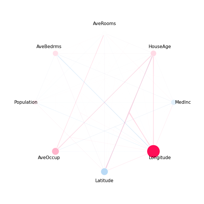
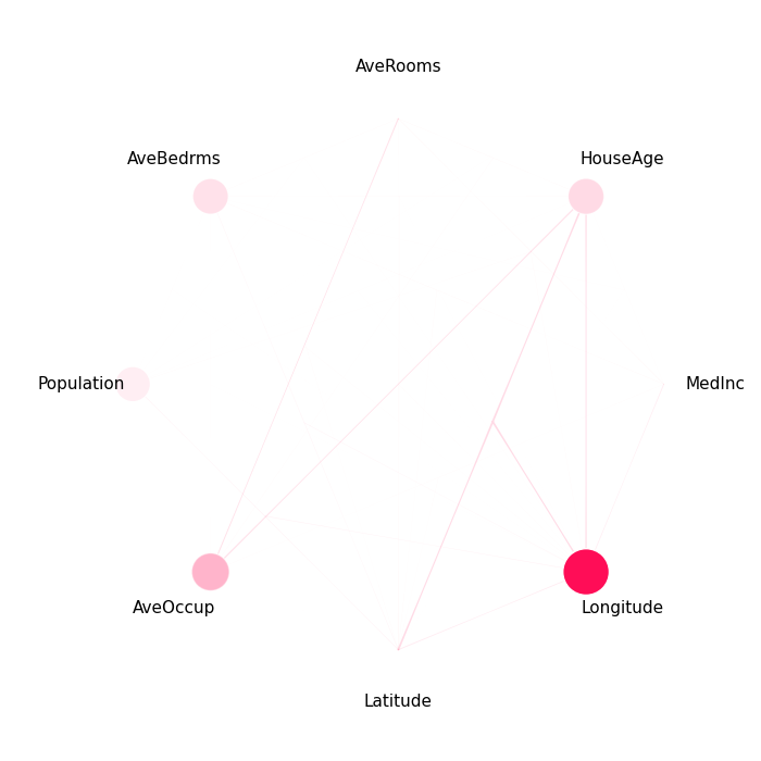
Scaling and Feature Names

Adjust node sizes and add feature names for readability.

explanation.plot_si_graph(
    feature_names=feature_names,
    size_factor=5.0,
    node_size_scaling=0.5,
)

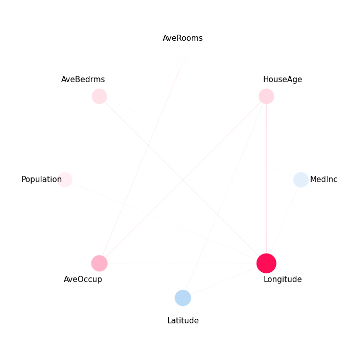
Filtering Interactions

Show only interactions above a threshold or the top-N strongest.

explanation.plot_si_graph(feature_names=feature_names, draw_threshold=0.05)

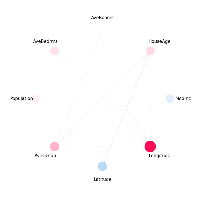
explanation.plot_si_graph(feature_names=feature_names, n_interactions=7)

explanation.plot_si_graph(feature_names=feature_names, interaction_direction="positive")

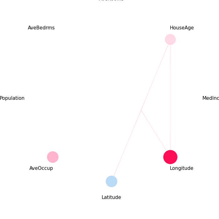
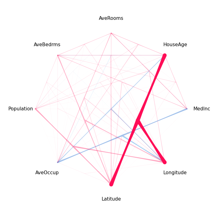
Filtering by Order

Show only interactions up to a certain order.

explanation.plot_si_graph(feature_names=feature_names, min_max_order=(1, 2))

explanation.plot_si_graph(feature_names=feature_names, min_max_order=(3, -1))